Lung cancer remains one of the leading causes of death worldwide due to its high rates of illness and mortality. In this study, we applied a continuous-time multi-state Markov model to examine how lung cancer progresses through six clinically defined stages, using retrospective data from 576 patients. The model describes movements between disease stages and the final stage (death), providing estimates of how long patients typically remain in each stage and how quickly they move to the next. It also considers important demographic and clinical factors such as age, smoking history, hypertension, asthma, and gender, which influence survival outcomes. Our findings show slower changes at the beginning of the disease but faster decline in later stages, with clear differences across patient groups. This approach highlights the dynamic course of the illness and can help guide tailored follow-up, personalized treatment, and health policy decisions. The study is based on a secondary analysis of publicly available data and therefore did not require clinical trial registration.

Keywords: 

lung cancer progression; multi-state Markov model; survival analysis

1. Introduction

Lung cancer is characterized by the uncontrolled proliferation of abnormal cells in the lungs, leading to major health challenges and life-threatening consequences [1]. It is one of the most common cancers worldwide, posing a primary public health concern in both incidence and mortality. In 2020, lung cancer was reported as the second most prevalent type of cancer, demanding urgent attention and coordinated action by the healthcare community [2,3].

It remains the leading cause of cancer-related morbidity and mortality [4], with outcomes largely linked to differences in smoking habits, less pronounced among women [5]. Tobacco smoking is the most critical determinant of lung cancer risk [6,7], with lifetime smokers facing far greater risk than non-smokers. Despite declining prevalence in countries such as the USA, smoking remains widespread in China and Eastern Europe, potentially generating tens of millions of new cases this century [8,9].

Epidemiological studies highlight the heavy burden of the disease. In Spain, a nationwide retrospective study (2010–2020) reported over 300,000 hospitalizations and approximately 70,500 deaths, underlining its clinical and economic impact [10]. Lung cancer also presents significant diagnostic and therapeutic challenges, although early detection substantially improves survival and treatment outcomes [11].

Given these challenges, robust statistical approaches are required to properly characterize disease dynamics. While traditional methods, such as Kaplan–Meier estimation and Cox regression, are useful for basic survival analysis, they are limited when applied to complex trajectories involving multiple intermediate states. In this context, multi-state models offer a promising framework to capture the heterogeneous progression patterns of lung cancer patients.

2. Materials and Methods

2.1. Lung Cancer

2.1.1. Basic Survival Analysis Concepts

Lung cancer can be split into two main types. The stage at which the cancer is found remains the most important factor of survival time, although factors such as geographic location and overall health also play significant roles. Various risk factors, including smoking and environmental exposures, increase the likelihood of developing lung cancer. Treatment options depend on the cancer stage, and advances in therapy and early detection have led to improved survival rates. Moreover, some patients can live for extended periods even with recurrent cancer due to better disease management.

2.1.2. Survival Analysis

Survival analysis is a statistical field focused on analyzing the time until a specific event occurs, such as death or relapse in cancer patients. Let T denote a non-negative random variable representing the time from diagnosis to the event (e.g., death). There are several approaches to survival analysis, including:

• The Kaplan–Meier estimator, which estimates the probability of survival over time while accounting for censored data.

• The Nelson–Aalen estimator, which estimates the cumulative hazard function over time, providing an alternative to the Kaplan–Meier for hazard-based interpretation.

• The Cox proportional hazards model, which examines how different factors affect the risk, assuming the ratio of risks stays the same between individuals is constant over time.

• Parametric models, which assume the time-to-event follows a specific distribution (e.g., exponential, Weibull, gamma, log-normal).

2.1.3. Survival and Hazard Functions

Definition 1 (Survival Function S(t)). Let T be a non-negative random variable representing time to an event (e.g., time from diagnosis to death). The survival function, 𝑆(𝑡), is the probability that an individual survives beyond time t. It is monotonically decreasing with 𝑆(0)=1 and lim𝑡→∞𝑆(𝑡)=0, and is defined as

𝑆(𝑡)=𝑃(𝑇>𝑡),𝑡≥0.

(1)

Definition 2 (Hazard Function h(t)). The hazard function, ℎ(𝑡), represents the instantaneous rate of failure at time t, conditional on survival until time t. It is defined as

ℎ(𝑡)=𝑓(𝑡)𝑆(𝑡),

(2)

where 𝑓(𝑡) is the probability density function.

2.1.4. Explanatory Variables

Factors that might affect survival are called explanatory variables or covariates. These can be fixed characteristics, such as gender or genetic marker, or time-varying factors, such as blood pressure or treatment status. Analyzing these variables is essential for understanding their impact on the survival outcomes.

In survival analysis, we seek to understand how these covariates affect the hazard and survival functions. For example, the Cox model is given by

ℎ(𝑡|𝑋=𝑥)=ℎ0(𝑡)exp(𝑥𝑇𝛽),

where ℎ0(𝑡) is the baseline hazard function (hazard for a reference group), x is the vector of covariates and 𝛽 is the vector of coefficients.

2.1.5. Multi-State Markov Models and the Markov Property

Multi-state Markov models extend traditional survival analysis by allowing for transitions between multiple states. The Markov property is a key assumption in these models, stating that the future state depends only on the present state and not on the sequence of events that preceded it. Mathematically, for a stochastic process {𝑋(𝑡),𝑡≥0} with state space S, the Markov property implies

𝑃(𝑋(𝑡𝑛+1)=𝑗|𝑋(𝑡𝑛)=𝑖,𝑋(𝑡𝑛−1)=𝑖𝑛−1,…,𝑋(𝑡1)=𝑖1)=𝑃(𝑋(𝑡𝑛+1)=𝑗|𝑋(𝑡𝑛)=𝑖),

(3)

for all times 𝑡1<𝑡2<…<𝑡𝑛<𝑡𝑛+1 and all states 𝑖1,𝑖2,…,𝑖𝑛−1,𝑖,𝑗∈𝑆.

This assumption has important implications and limitations in real clinical data, including:

• It simplifies the mathematical modeling but may not fully capture the complexity of disease progression

• It assumes that the time spent in the current state does not affect transition probabilities (memoryless property)

• In reality, the duration of illness or time since diagnosis often influences future progression

• Patient history and previous treatments may impact future transitions in ways not captured by the Markov property

• Semi-Markov models or hidden Markov models may be more appropriate when the Markov assumption is violated

Despite these limitations, Markov models provide a tractable framework for analyzing complex disease progressions and have proven valuable in clinical applications.

2.1.6. Dataset Description

This study analyzed retrospective patient data on lung cancer, focusing on individuals from 15 countries: Austria, Belgium, Bulgaria, Denmark, Finland, France, Germany, Ireland, Italy, Netherlands, Poland, Portugal, Romania, Spain, and Sweden. The dataset was obtained from a publicly accessible repository (Kaggle, https://www.kaggle.com/). For the purpose of this study, we considered only the subset of patients corresponding to these 15 countries. The research was designed to examine factors that may influence cancer prognosis and treatment outcomes by adopting a continuous-time homogeneous multi-state model for lung cancer mortality and survival progression. To operationalize this model, lung cancer progression was mapped into clinically defined stages, as shown in Table 1.

Table 1. Different stages of lung cancer and derived states.

The database that we considered contains demographic and clinical information, with basic details about the patients, organized as follows:

• Medical History: This section includes information about each patient’s medical background, such as smoking status (26.4% current smokers, 23.6% former smokers, 25.0% never smoked, and 25.0% passive smokers), Body Mass Index (mean = 30.26, SD = 8.40), and the presence of other health conditions such as hypertension (74.3%), asthma (49.8%), cirrhosis (25.7%), and other cancers (11.1%). It is crucial to identify potential risk factors and comorbidities.

• Cancer Diagnosis: Detailed data about the cancer diagnosis itself, including the stage of cancer at the time of diagnosis (Stage I: 25.9%, Stage II: 25.9%, Stage III: 25.2%, Stage IV: 23.1%). These variables are critical for tracking the progression and severity of the disease.

• Treatment Details: Information about the type of treatment each patient received (Chemotherapy: 25.9%, Radiation: 26.2%, Surgery: 25.9%, Combined: 22.0%), along with end date of the treatment, and the outcome (21.0% survived, 79.0% did not survive).

2.1.7. Missing Data and Censoring

The dataset contained no missing values across the included variables. This completeness allowed for robust analysis without the need for imputation methods. With respect to censoring, 21.0% of patients were right-censored because they were still alive at the end of the study period, while the remaining 79.0% experienced the event of interest (death). The distribution of patients across countries was balanced, ranging from 4.5% (Sweden) to 9.7% (Ireland) of the total sample. The mean age of patients was 54.9 years (SD = 10.1), with an age range of 28.0 to 90.0 years.

2.1.8. Ethical Considerations

This study is a retrospective secondary analysis of a publicly available, de-identified dataset. As such, no Institutional Review Board approval or patient consent was required, in accordance with the Declaration of Helsinki guidelines. All data were fully anonymized prior to analysis, and no identifiable information was used. Therefore, clinical trial registration was not applicable.

2.2. Statistical Analysis

All statistical analyses were peformed using SPSS version 27.0 (IBM Corp., Armonk, NY, USA). Descriptive statistics were reported using means and standard deviations for normally distributed continuous variables (e.g., age: 54.91 ± 10.07 years; BMI: 30.26 ± 8.40), and as frequencies with percentages for categorical variables (e.g., gender: 51.7% male, 48.3% female).

2.3. Multi-State Model

Lung cancer progression was represented using a continuous-time multi-state Markov process, defined over six clinically meaningful states corresponding to the TNM classification system [12]. Five of these states are transient, reflecting stages where patients may progress or regress, while the sixth state is absorbing, representing death. This alignment ensures that the mathematical structure mirrors the actual clinical trajectory.

Traditional survival methods, such as the Kaplan–Meier estimator and Cox proportional hazards regression, are limited when analyzing complex disease pathways involving multiple intermediate stages. They cannot provide state-specific transition probabilities or incorporate time-dependent covariates. In contrast, the multi-state Markov model allows: (1) modeling of complex progression pathways, (2) estimation of transition intensities between states, (3) incorporation of time-varying covariates, (4) calculation of state-specific survival probabilities and expected sojourn times, and (5) representation of heterogeneous clinical patterns observed in real patient cohorts.

Formally, the process is defined over the finite state space 𝑆={1,2,…,6}. It is characterized by a transition intensity matrix Q, where each off-diagonal entry 𝜆𝑖𝑗≥0 represents the instantaneous rate of transition from state i to state j, and each diagonal entry 𝜆𝑖𝑖=−∑𝑗≠𝑖𝜆𝑖𝑗 ensures that rows sum to zero. This framework allows precise estimation of expected times in each state, state-specific transition probabilities, and the overall dynamics of lung cancer progression.

To model disease progression, we employed a continuous-time homogeneous Markov process, defined over a finite state space 𝑆={1,2,…,6}, where each state represents a distinct clinical stage. The process is characterized by a transition intensity matrix Q, where each off-diagonal entry 𝜆𝑖𝑗≥0 represents the instantaneous rate of transition from state i to state j, and each diagonal entry 𝜆𝑖𝑖=−∑𝑗≠𝑖𝜆𝑖𝑗 ensures rows sum to zero.

𝑄=⎡⎣⎢⎢⎢⎢⎢⎢⎢⎢−𝜆11𝜆21𝜆31𝜆41𝜆510𝜆12−𝜆22𝜆32𝜆42𝜆520𝜆13𝜆23−𝜆33𝜆43𝜆530𝜆14𝜆24𝜆34−𝜆44𝜆540𝜆15𝜆25𝜆35𝜆45−𝜆550𝜆16𝜆26𝜆36𝜆46𝜆560⎤⎦⎥⎥⎥⎥⎥⎥⎥⎥.

Here, 𝜆𝑖𝑗≥0 for 𝑖≠𝑗, and 𝜆𝑖𝑖=−∑𝑗≠𝑖𝜆𝑖𝑗, ensuring that each row sums to zero. State 6 is an absorbing state, meaning once entered, no further transitions occur; thus, 𝜆6𝑗=0 for all j.

The transition probability matrix 𝑃(𝑡)=[𝑃𝑖𝑗(𝑡)] gives the probability of being in state j at time t given that the process started in state i. These probabilities satisfy the following Kolmogorov differential equations:

𝑑𝑃(𝑡)𝑑𝑡=𝑄𝑃(𝑡),(forwardequation)

𝑑𝑃(𝑡)𝑑𝑡=𝑃(𝑡)𝑄,(backwardequation)

with initial condition 𝑃(0)=𝐼, where I is the identity matrix. The general solution is obtained via the matrix exponential as

𝑃(𝑡)=exp(𝑄𝑡)=∑𝑘=0∞(𝑄𝑡)𝑘𝑘!.

This matrix exponential provides the transition probabilities for all state pairs over time t.

Theorem 1

(Uniqueness of the solution to the Kolmogorov equations). The matrix exponential 𝑃(𝑡)=exp(𝑄𝑡) is the unique solution to the Kolmogorov equations with the initial condition 𝑃(0)=𝐼.

Proof.  Let 𝑃(𝑡)=exp(𝑄𝑡). We need to show that this satisfies both the forward equation and the initial condition. First, for the initial condition:

𝑃(0)=exp(𝑄·0)=exp(0)=𝐼.

For the forward equation, we differentiate 𝑃(𝑡) with respect to t, obtaining

𝑑𝑑𝑡𝑃(𝑡)==𝑑𝑑𝑡exp(𝑄𝑡)=𝑑𝑑𝑡∑𝑘=0∞(𝑄𝑡)𝑘𝑘!=∑𝑘=1∞𝑄·𝑘·(𝑄𝑡)𝑘−1𝑘!𝑄∑𝑘=1∞(𝑄𝑡)𝑘−1(𝑘−1)!=𝑄∑𝑗=0∞(𝑄𝑡)𝑗𝑗!(𝑗=𝑘−1)=𝑄exp(𝑄𝑡)=𝑄𝑃(𝑡).

(4)

Thus, 𝑃(𝑡)=exp(𝑄𝑡) satisfies the forward equation. A similar derivation shows it also satisfies the backward equation.To prove uniqueness, suppose there exists another solution 𝑅(𝑡) that satisfies the forward equation with 𝑅(0)=𝐼. Define 𝑆(𝑡)=𝑅(𝑡)exp(−𝑄𝑡). Then

𝑑𝑑𝑡𝑆(𝑡)==𝑑𝑑𝑡[𝑅(𝑡)exp(−𝑄𝑡)]=𝑑𝑑𝑡𝑅(𝑡)·exp(−𝑄𝑡)+𝑅(𝑡)·𝑑𝑑𝑡exp(−𝑄𝑡)𝑄𝑅(𝑡)exp(−𝑄𝑡)−𝑅(𝑡)𝑄exp(−𝑄𝑡)=[𝑄𝑅(𝑡)−𝑅(𝑡)𝑄]exp(−𝑄𝑡).

(5)

Since 𝑅(𝑡) satisfies the forward equation, 𝑄𝑅(𝑡)=𝑅(𝑡)𝑄, so 𝑑𝑑𝑡𝑆(𝑡)=0. This means 𝑆(𝑡) is constant, and since 𝑆(0)=𝑅(0)exp(−𝑄·0)=𝐼·𝐼=𝐼, we have 𝑆(𝑡)=𝐼 for all t. Therefore, 𝑅(𝑡)=exp(𝑄𝑡)=𝑃(𝑡), proving uniqueness. □The expected time spent in a transient state j before absorption is given by

𝐸[𝑇𝑗]=∫∞0𝑃𝑗𝑗(𝑡)𝑑𝑡.

Under the assumption that the sojourn time in state j follows an exponential distribution with rate −𝜆𝑗𝑗, hence

𝑃𝑗𝑗(𝑡)=𝑒𝜆𝑗𝑗𝑡,where𝜆𝑗𝑗<0.

Then,

𝐸[𝑇𝑗]=∫∞0𝑒𝜆𝑗𝑗𝑡𝑑𝑡=[1𝜆𝑗𝑗𝑒𝜆𝑗𝑗𝑡]∞0=−1𝜆𝑗𝑗.

For a more general analysis of absorption properties, we can partition the transition intensity matrix Q as

𝑄=[𝑇0𝐴0],

where T is the sub-matrix corresponding to transitions between transient states, A contains rates of absorption, and the bottom row of zeros reflects the absorbing state property.

The fundamental matrix 𝑁=(−𝑇)−1 plays a crucial role in analyzing absorption properties. The entry 𝑁𝑖𝑗 represents the expected number of visits to state j starting from state i before absorption.

Theorem 2 (Expected Time to Absorption). The expected time to absorption starting from transient state i, denoted 𝜇𝑖, is given by:

𝜇𝑖=∑𝑗𝑁𝑖𝑗,

where the sum is over all transient states j.Proof.  Let 𝜇𝑖 be the expected time to absorption starting from state i. By conditioning on the first transition, we have

𝜇𝑖=1−𝜆𝑖𝑖+∑𝑗≠𝑖,𝑗 transient𝜆𝑖𝑗−𝜆𝑖𝑖𝜇𝑗.

The first term represents the expected time spent in state i before any transition, and the second term accounts for transitions to other transient states.Rearranging the equation abouve, we obtain

−𝜆𝑖𝑖𝜇𝑖=1+∑𝑗≠𝑖,𝑗transient𝜆𝑖𝑗𝜇𝑗.

This can be written in matrix form as 𝑇𝝁=−𝟏, where 𝝁 is the vector of expected times to absorption and 𝟏 is a vector of ones. Therefore, 𝝁=−𝑇−1𝟏=𝑁𝟏, which gives 𝜇𝑖=∑𝑗𝑁𝑖𝑗. □

Variance of Time to Absorption

Beyond expected values, we can also derive the variance of the time to absorption.

Theorem 3 (Variance of Time to Absorption). The variance of the time to absorption starting from state i, denoted 𝜎2𝑖, is given by

𝜎2𝑖=2∑𝑗𝑁(2)𝑖𝑗−𝜇2𝑖,

where 𝑁(2)=𝑁·𝑑𝑖𝑎𝑔(𝑁) and 𝑑𝑖𝑎𝑔(𝑁) is a diagonal matrix with the same diagonal entries as N.Proof.  Let 𝑀𝑖(𝑠) be the moment generating function of the time to absorption starting from state i. It can be shown that

𝑀𝑖(𝑠)=[(𝑠𝐼−𝑇)−1𝐴𝟏]𝑖.

The first and second moments can be derived by differentiating 𝑀𝑖(𝑠) with respect to s and evaluating at 𝑠=0 are

𝜇𝑖=𝑀′𝑖(0)=[(−𝑇)−1𝟏]𝑖=∑𝑗𝑁𝑖𝑗,

and

𝐸[𝑇2𝑖]=𝑀″𝑖(0)=[2(−𝑇)−2𝟏]𝑖=2∑𝑗𝑁(2)𝑖𝑗.

The variance is given by

𝜎2𝑖=𝐸[𝑇2𝑖]−𝜇2𝑖=2∑𝑗𝑁(2)𝑖𝑗−𝜇2𝑖.   □

2.4. Likelihood Function

Suppose the k-th individual is observed at time points 𝑡(𝑘)1<𝑡(𝑘)2<⋯<𝑡(𝑘)𝑚𝑘, with corresponding states 𝑠(𝑘)1,𝑠(𝑘)2,…,𝑠(𝑘)𝑚𝑘. The likelihood contribution from this trajectory is

𝐿(𝑘)(𝑄)=∏𝑙=1𝑚𝑘−1[exp(𝑄(𝑡(𝑘)𝑙+1−𝑡(𝑘)𝑙))]𝑠(𝑘)𝑙,𝑠(𝑘)𝑙+1.

Assuming independence across N individuals, the full likelihood is given by

𝐿(𝑄)=∏𝑘=1𝑁𝐿(𝑘)(𝑄)=∏𝑘=1𝑁∏𝑙=1𝑚𝑘−1[exp(𝑄(𝑡(𝑘)𝑙+1−𝑡(𝑘)𝑙))]𝑠(𝑘)𝑙,𝑠(𝑘)𝑙+1.

The log-likelihood function is then

ℓ(𝑄)=∑𝑘=1𝑁∑𝑙=1𝑚𝑘−1log([exp(𝑄(𝑡(𝑘)𝑙+1−𝑡(𝑘)𝑙))]𝑠(𝑘)𝑙,𝑠(𝑘)𝑙+1).

The transition probability matrix exp(𝑄𝑡) is evaluated numerically, and maximum likelihood estimation is employed to estimate the intensity parameters 𝜆𝑖𝑗. Since closed-form expressions for the likelihood are unavailable in most practical cases, numerical optimization algorithms are utilized for parameter inference.

The continuous-time homogeneous Markov model incorporated both time-fixed and time-dependent covariates. The time-fixed covariates included age (mean = 54.9 years), gender (51.7% male, 48.3% female), and country of origin, which were assumed not to change over time. In addition, time-dependent covariates, namely smoking status (26.4% current smokers, 23.6% former smokers, 25.0% never smoked, and 25.0% passive smokers), BMI (mean = 30.3), and treatment modality (Chemotherapy: 25.9%, Radiation: 26.2%, Surgery: 25.9%, Combined: 22.0%) were incorporated as time-dependent covariates, updated at each clinical assessment.

Covariates were integrated into the model by allowing them to affect the transition intensities through a proportional hazards approach

𝑞𝑟𝑠(𝑡,𝐳(𝑡))=𝑞(0)𝑟𝑠exp(𝜷𝑇𝑟𝑠𝐳(𝑡)),

(6)

where 𝑞𝑟𝑠(𝑡,𝐳(𝑡)) is the transition intensity from state r to state s at time t with covariate vector 𝐳(𝑡), 𝑞(0)𝑟𝑠 is the baseline transition intensity, and 𝜷𝑟𝑠 is the vector of regression coefficients specific to the transition from state r to state s. The transition probability matrix exp(𝑄𝑡) is evaluated numerically, and maximum likelihood estimation is employed to estimate the intensity parameters 𝜆𝑖𝑗. Numerical optimization algorithms are utilized for parameter inference.

3. Results

The study included 576 patients diagnosed with lung cancer. Table 2, Table 3 and Table 4 present the descriptive statistics for demographic and clinical characteristics. The mean age of patients was 54.9 years (SD = 10.1), ranging from 28.0 to 90.0 years, and 51.7% were male. At baseline, 26.4% of patients were current smokers, 23.6% were former smokers, 25.0% had never smoked, and 25.0% were passive smokers. The distribution of cancer stages at diagnosis was relatively balanced, with Stage I at 25.9%, Stage II at 25.9%, Stage III at 25.2%, and Stage IV at 23.1%. A family history of cancer was reported in 46.2% of patients. Comorbidities were hypertension (74.3%), asthma (49.8%), cirrhosis (25.7%), and other cancers (11.1%).

Table 2. Demographic characteristics of the study population.

Table 3. Descriptive statistics for continuous variables.

Table 4. Percentiles for continuous variables.

Survival analysis was performed using the Kaplan–Meier method to estimate time-to-event functions across patients subgroups. The impact of age, gender, and clinical risk factors on survival outcomes were subsequently evaluated.

• According to Figure 1, survival probability decreased with increasing age. Patients over 80 years exhibited a pronounced decline in survival, and female patients maintained higher survival probabilities after age 80 compared to males.

• Interestingly, patients with a history of hypertension or asthma demonstrated better survival, which may reflect more frequent monitoring and earlier interventions (see Figure 2 and Figure 3).

• Cirrhosis patients and current smokers experienced significantly reduced survival, particularly after the age of 80, higlighting these factors as critical risks (see Figure 4 and Figure 5).

These findings underscore the importance of demographic and clinical determinants of survival and will guide covariate selection in subsequent multistate modeling.

Mean Waiting Time Analysis

Table 5 presents the estimated mean sojourn times (i.e., expected waiting times) in each transient state before transitioning to another state within the multi-state Markov model. These estimates quantify the average duration lung cancer patients remain in each disease stage prior to progression.

Table 5. Estimated mean sojourn times in transient states.

The longest mean waiting time was observed in state 1 (5.8 years), suggesting a relatively stable or indolent early disease phase. States 3 and 5 also exhibited prolonged waiting times, indicating delayed transitions and possibly reflecting clinical states with slower progression or effective symptom control. In contrast, the shortest mean duration occurred in state 2 (1.0 years), implying a higher rate of progression to subsequent states, consistent with a more unstable or rapidly evolving disease stage. Similarly, state 4 showed a shorter mean waiting time (1.5 years), often transitioning quickly to state 5. Notably, state 5, just prior to the absorbing state (state 6, representing death), had a mean waiting time of 3.6 years. This interval provides insight into the disease burden and survival potential before terminal.

Figure 1. Kaplan–Meier estimates of the survival function regarding the patient’s age and gender.

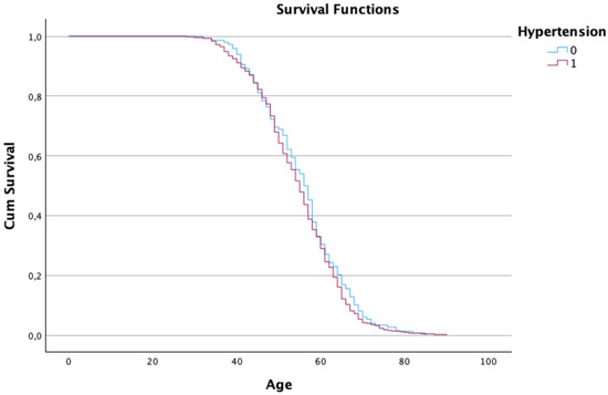
Figure 2. Kaplan–Meier estimates of the survival function regarding the patient’s age and hypertension.

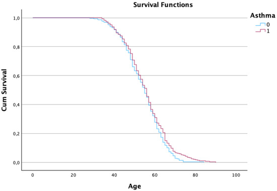
Figure 3. Kaplan–Meier estimates of the survival function regarding the patient’s age and asthma condition.

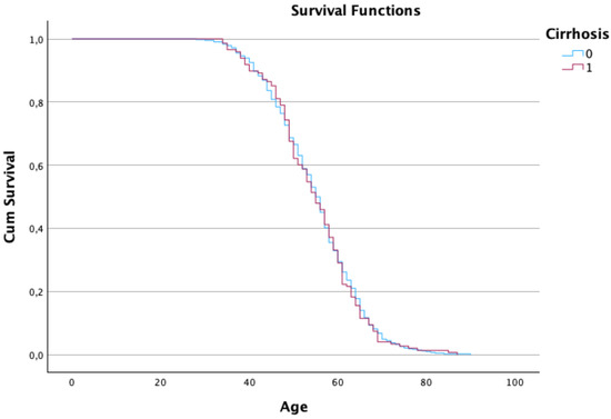
Figure 4. Kaplan–Meier estimates of the survival function regarding the patient’s age and cirrhosis condition.

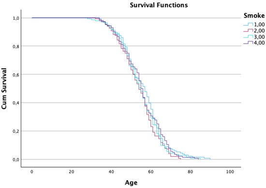
Figure 5. Kaplan–Meier estimates of the survival function regarding the patient’s age and smoking status.

4. Discussion

Lung cancer remains a major global health burden, with substantial morbidity and mortality worldwide. Despite advances in treatment, outcomes are poor unless the disease is detected early and managed effectively [13,14]. Early diagnosis improves prognosis and survival, emphasizing the importance of proactive prevention, screening, and timely intervention by health organizations [13,15].

We employed a continuous-time, time-homogeneous multi-state Markov model to characterize lung cancer progression across six clinically meaningful stages, with states 1–5 transient and state 6 representing death. This framework allows estimation of clinically relevant quantities such as state occupancy probabilities, transition intensities, and expected sojourn times, providing a rigorous depiction of disease dynamics and supporting personalized clinical decision-making [16,17].

Our findings indicate heterogeneous disease trajectories. Patients remained longest in state 1 (mean sojourn 5.8 years), whereas state 2 showed rapid progression (mean 1.0 year). State 3 also exhibited prolonged occupancy, while patients in state 5 reached the absorbing state in an average of 3.6 years. These results highlight stage-specific progression patterns and the clinical severity of advanced disease. Observed patterns align with prior studies, including [18], which reported elevated transition probabilities to distant metastasis within two years post-surgery in stage IIB patients.

Demographic and clinical covariates further influenced survival. Kaplan–Meier analyses revealed declining survival with age, yet females over 80, hypertensive, or asthmatic patients exhibited relatively longer survival, whereas current smokers experienced poorer outcomes [19]. These insights underscore the importance of individual-level factors in shaping disease trajectories and the potential for targeted interventions.

Clinically, the model-derived state-dependent transition probabilities can inform risk-adapted surveillance strategies. For example, older patients with a smoking history may require closer follow-up due to faster progression, whereas younger non-smokers may benefit from less intensive monitoring. Stage-specific sojourn times can guide timely therapy escalation or prioritization of more aggressive interventions in patients at higher risk of rapid deterioration. While these applications are exploratory, they demonstrate how multi-state modeling can translate statistical insights into actionable clinical guidance. Our study illustrates that multi-state Markov models provide a comprehensive view of lung cancer progression, integrating clinical and demographic covariates to inform patient-specific care and support evidence-based healthcare planning.

5. Conclusions

The application of a continuous-time multi-state Markov model enabled a nuanced analysis of lung cancer progression across clinically distinct disease states. Our findings show that lung cancer exhibits a slow initial progression from state 1, with a mean waiting time of 5.8 years, but accelerates notably in state 2. The final transition to death from state 5 occurred in a mean time of 3.6 years. These temporal dynamics reflect the complex nature of disease evolution and underscore the importance of timely intervention.

Demographic and clinical variables significantly modulated survival. Patients over 80 years of age who were female or had comorbid hypertension or asthma tended to live longer, whereas those with active smoking status experienced accelerated mortality. These findings corroborate recent epidemiological evidence and emphasize the role of lifestyle and comorbidity management in improving lung cancer outcomes [19].

Ultimately, the insights from this model can guide personalized surveillance strategies, inform health economic evaluations, and support clinical decision-making. Early detection and stratified treatment remain pivotal, particularly given the observed variation in progression rates across states. Multi-state modeling thus provides a powerful framework to translate real-world data into actionable strategies for improving lung cancer care.

6. Limitations

This study is limited by its reliance on a retrospective cohort of 576 patients, which may constrain the generalizability of the findings. Future studies should consider larger, multicenter datasets to enhance statistical power and external validity. Moreover, this model focused solely on death as the absorbing outcome. Inclusion of additional competing events such as metastasis, recurrence, or secondary malignancies would yield a more granular and clinically relevant understanding of disease progression.

A limitation of this study is that we did not perform formal internal or external validation of the proposed multi-state model. While the estimates were derived using rigorous likelihood-based methods, their robustness could be further assessed through internal validation strategies such as bootstrap resampling or cross-validation, which allow for the evaluation of variability and potential overfitting. Similarly, external validation with an independent cohort would provide stronger evidence of generalizability. Such validation was not feasible due to data availability, but we highlight it as an important direction for future work.

Author Contributions

All Conceptualization, V.R. and S.S.F.; methodology and formal analysis, V.R.; validation, S.S.F. and D.F.; writing—original draft, V.R.; writing—review and editing, S.S.F. and A.A.; supervision, S.S.F. and A.A. All authors have read and agreed to the published version of the manuscript.

Funding

This work was partially supported by the Portuguese Foundation for Science and Technology through the projects UIDB/00212/2020, UIDB/04630/2020 and UIDB/00297/2020.

Data Availability Statement

The dataset supporting this analysis is available from Kaggle (https://www.kaggle.com/). Modified versions of the dataset during the current study are available from the corresponding author on reasonable request.

Acknowledgments

The authors would like to thank the anonymous reviewers and the Associate Editor for their comments and suggestions, which have greatly improved the quality of this manuscript.

Conflicts of Interest

The authors declare no conflicts of interest.

References

1. Gao, S.; Zhang, G.; Lian, Y.; Li, Y.; Gao, H. Exploration and analysis of the value of tumor-marker joint detection in the pathological type of lung cancer. Cell. Mol. Biol. 2020, 99, 93–97. [Google Scholar] [CrossRef]
2. World Health Organization. Cancer. Fact Sheets. Available online: https://www.who.int/news-room/fact-sheets/detail/cancer (accessed on 21 September 2024).
3. World Cancer Research Fund International. Lung Cancer Statistics. Available online: https://www.wcrf.org/cancertrends/lung-cancer-statistics/ (accessed on 21 September 2024).
4. Gottlin, E.B.; Bentley, R.C.; Campa, M.J.; Pisetsky, D.S.; Herndon, J.E.; Patz, E.F. The association of intratumoral germinal centers with early-stage non-small cell lung cancer. J. Thorac. Oncol. 2011, 6, 1687–1690. [Google Scholar] [CrossRef] [PubMed]
5. Sung, H.; Ferlay, J.; Siegel, R.L.; Laversanne, M.; Soerjomataram, I.; Jemal, A.; Bray, F. Global cancer statistics 2020: GLOBOCAN estimates of incidence and mortality worldwide. CA Cancer J. Clin. 2021, 71, 209–249. [Google Scholar] [CrossRef] [PubMed]
6. Caini, S.; Del Riccio, M.; Vettori, V.; Scotti, V.; Martinoli, C.; Raimondi, S.; Cammarata, G.; Palli, D.; Banini, M.; Masala, G.; et al. Quitting smoking at or around diagnosis improves lung cancer survival: A systematic review and meta-analysis. J. Thorac. Oncol. 2022, 17, 623–636. [Google Scholar] [CrossRef] [PubMed]
7. Wang, X.; Romero-Gutierrez, C.W.; Kothari, J.; Shafer, A.; Li, Y.; Christiani, D.C. Prediagnosis smoking cessation and overall survival among patients with non–small cell lung cancer. JAMA Netw. Open 2023, 6, e2311966. [Google Scholar] [CrossRef] [PubMed]
8. Parkin, D.M.; Bray, F.I.; Devesa, S. Cancer burden in the year 2000: The global picture. Eur. J. Cancer 2001, 37, 4–66. [Google Scholar] [CrossRef] [PubMed]
9. Peto, R.; Darby, S.; Deo, H.; Silcocks, P.; Whitley, E.; Doll, R. Smoking, smoking cessation, and lung cancer in the UK since 1950: Combination of national statistics with two case-control studies. BMJ 2000, 321, 323. [Google Scholar] [CrossRef] [PubMed]
10. Galindo-Utrero, A.; San-Román-Montero, J.M.; Gil-Prieto, R.; Gil-de-Miguel, A. Trends in hospitalization and in-hospital mortality rates among patients with lung cancer in Spain between 2010 and 2020. BMC Cancer 2022, 22, 1199. [Google Scholar] [CrossRef] [PubMed]
11. Zarbakhsh, P. Spatial attention in U-Net for breast tumor segmentation. Appl. Sci. 2023, 13, 8758. [Google Scholar] [CrossRef]
12. Goldstraw, P.; Chansky, K.; Crowley, J.; Rami-Porta, R.; Asamura, H.; Eberhardt, W.E.; Nicholson, A.G.; Groome, P.; Mitchell, A.; Bolejack, V.; et al. The IASLC lung cancer staging project: Proposals for revision of the TNM stage groupings in the forthcoming (eighth) edition of the TNM classification for lung cancer. J. Thorac. Oncol. 2016, 11, 39–51. [Google Scholar] [CrossRef] [PubMed]
13. Greene, C.M.; Abdulkadir, M. Global respiratory health priorities at the beginning of the 21st century. Eur. Respir. Rev. 2024, 33, 230205. [Google Scholar] [CrossRef] [PubMed]
14. Lam, D.C.; Liam, C.K.; Andarini, S.; Park, S.; Tan, D.S.; Singh, N.; Jang, S.H.; Vardhanabhuti, V.; Ramos, A.B.; Nakayama, T.; et al. Lung cancer screening in Asia: An expert consensus report. J. Thorac. Oncol. 2023, 18, 1303–1322. [Google Scholar] [CrossRef] [PubMed]
15. Shankar, A.; Dubey, A.; Saini, D.; Singh, M.; Prasad, C.P.; Roy, S.; Bharati, S.J.; Rinki, M.; Singh, N.; Seth, T.; et al. Environmental determinants of lung cancer. Transl. Lung Cancer Res. 2019, 8, S31–S49. [Google Scholar] [CrossRef] [PubMed]
16. Grover, G.; Sabharwal, A.; Kumar, S.; Thakura, A.K. A multi-state Markov model for the progression of chronic kidney disease. Turkiye Klinikleri J. Biostat. 2019, 11, 1–14. [Google Scholar] [CrossRef]
17. Lintu, M.K.; Shreyas, K.M.; Kamath, A. Multi-state model for kidney disease. Clin. Epidemiol. Glob. Health 2022, 13, 100946. [Google Scholar] [CrossRef]
18. Jeong, W.G.; Choi, H.; Chae, K.J.; Kim, J. Recurrence in early-stage lung cancer: A multistate model. Transl. Lung Cancer Res. 2022, 11, 1279–1291. [Google Scholar] [CrossRef] [PubMed]
19. Tesfaw, L.M.; Dessie, Z.G.; Mekonnen Fenta, H. Lung cancer mortality and associated predictors: Systematic review using 32 scientific research findings. Front. Oncol. 2023, 13, 1308897. [Google Scholar] [CrossRef] [PubMed]